The Data

This tool was trained on publicly available data gathered by The National Survey on Drug Use and Health (NSDUH) during the years 2015-2017. The NSDUH is a nationwide study providing information on tobacco, alcohol, drug-use, mental health, and other health-related issues in the general population of the United States. The study collects data via individual interviews with approximately 70,000 teens and adults each year and the results are used to inform various public health programs, policies, and tools such as this OMR-Tool. For more information on the survey, please visit their website:


NSDUH Website


Although the NSDUH data set dates back to 1971, using only recent data was a key design consideration. The opioid crisis has grown and changed rapidly in recent years, and it is important for the model to make its predictions based on the current state of the opioid crisis. Additionally, the survey underwent several changes starting in 2015, making earlier data difficult to integrate. For example, the recently updated Diagnostic and Statistical Manual of Mental Disorders (DSM-V) standards were incorporated into the survey in 2015, changing the diagnostic criteria for many of the included drug and mental health disorders. The raw data set contained approximately 170,000 rows, with each row corresponding to a different survey respondent (individual respondents are not allowed to take the survey more than once, in the same year or across multiple years). After removing participants who had not used prescription painkillers in the past year, the dataset contained approximately 53,000 respondents, making this value the effective N-size of the tool.

Feature Selection and Pre-Processing

The data set contains 2,631 features, each of which corresponds to either a question directly asked on the NSDUH survey, or a recoded variable created from aggregating multiple questions. The outcome variable for this tool is “Opioid Misuse”, defined as people who answered “Yes” to the question: “Have you ever, even once, used any prescription pain reliever in any way a doctor did not direct you to use it in the past 12 months?” This question is further defined to include using prescription pain relievers “without a prescription of your own”, “in greater amounts, more often, or longer than you were told to take it”, or “in any other way a doctor did not direct you to use it."


Each survey respondent was categorized as having misused or not misused opioids in the past 12 months (from the survey date). For variables that had only categorical responses, the team one-hot-encoded them before adding to the model. For variables with a mix of categorical and continuous responses (e.g., “At what age did you first smoke cigarettes” with an additional response option for “never smoked”), the continuous responses were first binned, and then one-hot-encoded along with the categorical responses.


Feature Reduction

One key challenge was to narrow down the feature space from 2,631 variables in the survey to roughly 25 variables/questions, which a patient could practically provide responses for on a form in a physician’s office. Several strategies for choosing or excluding features helped achieve this goal:


  1. Excluding features that were effectively asking the same question as the outcome variable.
  2. Excluding features that were very similar to other features in the same topic.
  3. Excluding features that only inquired about patient behaviors / activities in the past 30 days, as including these would have likely introduced significant look-ahead bias; since the outcome variable measured opioid misuse in the prior 12 months.
  4. Choosing feature categories based on what existing research has shown are the most likely contributors to opioid misuse: patient age, tobacco use, other substance abuse (hard drugs), mental health, etc.
  5. Choosing features with high differences of misuse prevalence across their response options. Since N-size can be so impactful to this type of calculation, computing the weighted standard deviation of misuse prevalence across response options for each question provided an automated and robust way to quickly evaluate each feature.
  6. Excluding features from existing research that did not have a strong difference in their prevalence of opioid misuse across response options.
  7. Excluding features with perfect or near-perfect correlation with other features, as this multicollinearity could be harmful to both model performance and feature importance accuracy.


Potential Look-Ahead Bias

Because both the outcome variable and certain misuse features for other drugs asked about usage in the previous 12 months, the team had to consider the possibility of look-ahead bias; that is, for individuals who misused both opioids and another substance in the previous 12 months, which of the misuses came first? Perhaps misusing opioids caused individuals to misuse other substances, which would mean misuse of the other drug would be an outcome rather than a feature; this case would lead to over-predicting risk for individuals who have used these other substances. However, it could also be the other way around, where other substance misuse came first and therefore is a legitimate predictor of opioid misuse. Or it could indicate an underlying predictor of a propensity to misuse opioids (e.g., a patient with an “addictive personality”), regardless of which one came first.


To deal with this potential bias, when possible, the team selected features that encompassed wider time-frames than the 12-month misuse window. This tactic was not always possible, but the direction of the look-ahead bias erred on the side of over-predicting risk, which was the more conservative and therefore more tolerable direction of bias. This was one of the main reasons why the team was okay allowing a few features with this potential bias. If this project advances to the clinical trials stage, the team will prioritize eliminating look-ahead bias in a designed experiment.


In conclusion, while there is potentially look-ahead bias, it is by no means definitive, nor is it a detractor of this project’s effectiveness. Given the few features impacted and conservative direction of the potential bias, along with the opportunity to eliminate it in future stages, the team accepted this risk but also felt it was important to acknowledge.

Model Selection and Evaluation

The model was trained using 60% of the ~53,000 row dataset. 25% of the data was used for calibration and validation, retaining the remaining 15% of the data as a test set.


Model Selection

The team experimented with numerous models of various complexity, starting with a simple logistic regression model, which served as a parsimonious baseline against which other models could be compared. The next model attempted was an Extreme Gradient Boost (XG Boost or XGB) model, an implementation of gradient boosted decision trees known to work particularly well for the relatively small-sized, dense data used in this project. Finally, to experiment with a completely different family of models, the team constructed a simple neural network.


All three of these initial models were “uncalibrated”, with XG Boost performing considerably better than the other two (see Model Evaluation subsection below for our evaluation criteria). To further improve model performance, models were run through a calibrated classifier, which is specifically designed to improve the quality of the models' predicted probabilities. This resulted in three additional calibrated versions of the models, all of which performed slightly better than the uncalibrated XG Boost model, and which were all similar in performance.


Ordinarily, "black box" models such as XG Boost and neural networks have the undesirable tradeoff of sacrificing interpretability for performance. However, the use of Shapley values (see Shapley values section below) to communicate personalized feature importance enables physicians to interpret which features increase or decrease a patient’s risk score, something the team deemed vital for tool usefulness and adoption.


Model Evaluation

Brier Loss Score was the primary evaluation metric used to assess model performance. Though perhaps not as well-known as other evaluation metrics for binary classification, it has been used since 1950. Brier Loss Score is a practical method for this use case because it is specifically designed for probability evaluation. For example, in a group of 100 patients, all of whom have a predicted probability of approximately 20%, Brier Loss Score will indicate the best performance when 20 of those patients actually misused opioids and 80 did not. It is important to remember, unlike is often the case of binary classification problems, the goal of this project is to predict the probability of opioid misuse rather than the binary outcome of a patient misusing or not misusing opioids. Therefore, traditional model evaluation techniques such as Precision, Recall, F1 Score, and ROC AUC metrics were not helpful in evaluating desired probability outputs, as they focus on ratios of false positives and false negatives as opposed to measuring probability.


The team also generated calibration curves (a.k.a., reliability diagrams) from the test data for each model, which compare the relative frequency of what was observed to the predicted probability frequency. While the best models are closest to the diagonal line, which represents a perfectly calibrated model (each probability predicted by the model is exactly correct), since no model is perfect, the team preferred models whose bias overestimated risk (the safe zone) rather than underestimated risk (the danger zone). The diagram below depicts model performance on these calibration curves.


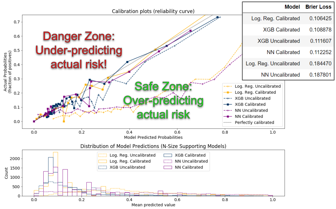
In all the top performing models (those closest to the diagonal line), even at their worst performance, the predicted probabilities are only roughly seven percentage points away from the actual probabilities, a good practical validation of model performance.


Additionally, the histogram shown below the calibration plot shows a similar distribution among the calibrated models, with most patients scoring between 0% and 20% likelihood of opioid misuse, and the long right tail showing few people scoring higher.


Final Model

The final model chosen for the OMR Tool is a calibrated XG Boost model. While the calibrated logistic regression model had a slightly lower Brier Loss Score, the team ultimately chose the calibrated XG Boost model because it incorporates feature interaction, making the personalized feature importance output (see Shapley Value section below) far more aligned with existing literature. An example of the distribution of feature importance of the calibrated Logistic Regression model compared to the calibrated XG Boost model is shown below.


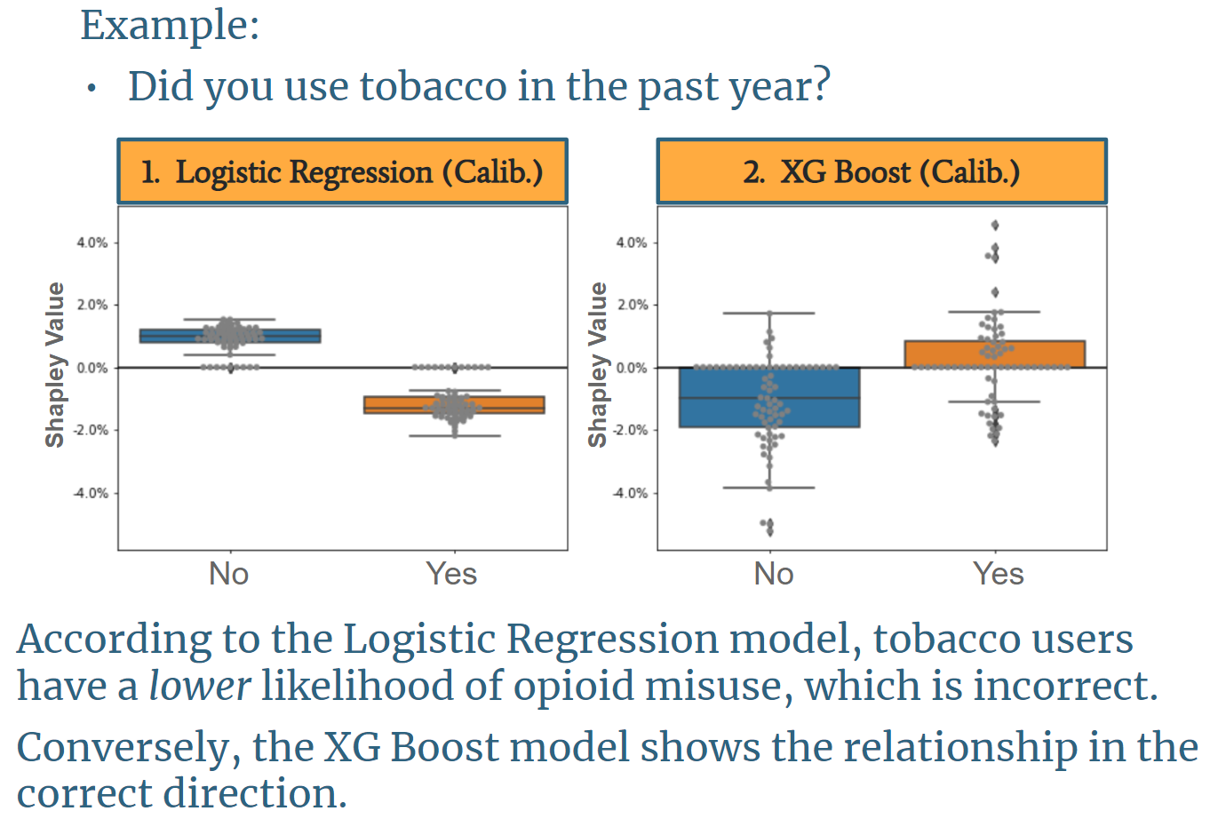
The image above is based on a question asking if a user has smoked tobacco in the past year. It shows with logistic regression, tobacco users are less likely to misuse opioids, and non-tobacco users are more likely to misuse opioids. This finding is counterintuitive, misaligned with existing research, and misaligned with the underlying data. Conversely, the XG Boost model shows the correct direction of impact on opioid risk.


Shapley Values

It is important for a physician to know why each patient receives their particular risk score. While this task is a straightforward output for a simple uncalibrated logistic regression model, as model complexity increases, human understanding of the model typically decreases. To add clarity for our users and to help physicians understand the risk for each of their patients individually, the OMR-Tool provides a visual output of each user’s top five features (i.e., patient answers to each question) that contributed most to their total risk score, displayed as a two-sided bar graph. A Shapley value shows how much each feature contributes to the overall risk score. Mathematically, a Shapley value is the average marginal contribution of a feature value across all possible combinations of features from our model. For one patient, their previous non-opioid substance abuse may have been the primary feature that brought their risk score up, but for another patient, even if they also have the same history of non-opioid substance abuse, it could be the simple fact of, for example, being young and male that contributed most to their individual risk. Each patient is different, and the tool assesses each individual’s information holistically, rather than statically question by question as in previous risk assessment tools.


It is important to note, however, that this tool does not claim experimental causality between the features and opioid misuse; rather, it is claiming predictive association between the features and opioid misuse. For example, it would be technically incorrect to say that being young and male causes a patient’s risk score to go up, but it is acceptable to say that being young and male is predictive of and/or contributes to a patient’s high risk score. While achieving causal proof of the relationship between features and opioid misuse is ideal, the experiment required to achieve this claim is infeasible for many reasons. Moreover, there is a long precedent in the medical world to use predictive association, as illustrated when a physician asks if a patient has a family history of some condition. While family history can be predictive of a condition, it doesn’t mean that it has been causally proven to drive that same condition, yet physicians frequently use it as an indicator of patient risk for that condition.

Production Pipeline

Our OMR Assessment is delivered via a multi-step webform that we developed using Django, a python web-framework. Upon submission, our solution pre-processes the webform responses and feeds them into our trained, calibrated XG Boost model and evaluation scripts. Our scripts output three important pieces of information: the likelihood of the patient to misuse opioids, the corresponding percentile for that likelihood within the general population, and personalized feature importance through use of Shapley values. These three data objects are inputs for our patient risk report and data visualizations. Fusion Charts, a JavaScript charting library, are used for building the data visualizations. Lastly, Bootstrap components are used to render the charts and corresponding data tables on the OMR Report, which a physician can reference when meeting with the patient.